1.17. Neural network models (supervised)

Warning

This implementation is not intended for large-scale applications. In particular,scikit-learn offers no GPU support. For much faster, GPU-based implementations,as well as frameworks offering much more flexibility to build deep learningarchitectures, see Related Projects.

1.17.1. Multi-layer Perceptron

Multi-layer Perceptron (MLP) is a supervised learning algorithm that learnsa function

by training on a dataset,where is the number of dimensions for input and is thenumber of dimensions for output. Given a set of featuresand a target, it can learn a non-linear function approximator for eitherclassification or regression. It is different from logistic regression, in thatbetween the input and the output layer, there can be one or more non-linearlayers, called hidden layers. Figure 1 shows a one hidden layer MLP with scalaroutput.

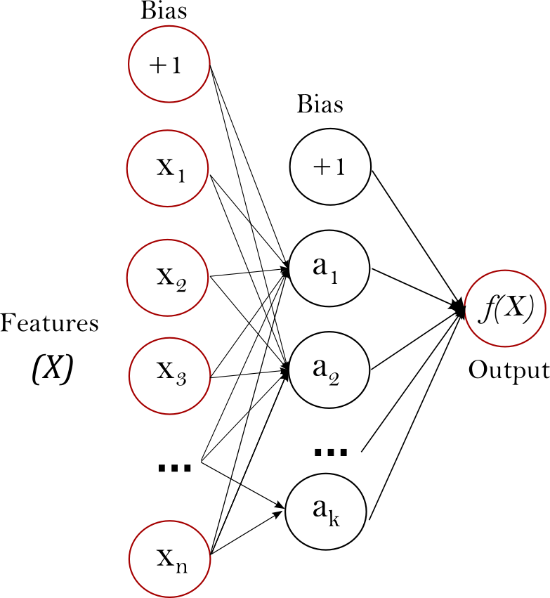Figure 1 : One hidden layer MLP.

The leftmost layer, known as the input layer, consists of a set of neurons

representing the input features. Eachneuron in the hidden layer transforms the values from the previous layer witha weighted linear summation, followedby a non-linear activation function

• likethe hyperbolic tan function. The output layer receives the values from thelast hidden layer and transforms them into output values.

The module contains the public attributes coefs and intercepts.coefs_ is a list of weight matrices, where weight matrix at index

represents the weights between layer and layer. intercepts_ is a list of bias vectors, where the vectorat index represents the bias values added to layer.

The advantages of Multi-layer Perceptron are:

• Capability to learn non-linear models.

• Capability to learn models in real-time (on-line learning)using partial_fit.

The disadvantages of Multi-layer Perceptron (MLP) include:

• MLP with hidden layers have a non-convex loss function where there existsmore than one local minimum. Therefore different random weightinitializations can lead to different validation accuracy.

• MLP requires tuning a number of hyperparameters such as the number ofhidden neurons, layers, and iterations.

• MLP is sensitive to feature scaling.

Please see Tips on Practical Use section that addressessome of these disadvantages.

1.17.2. Classification

Class MLPClassifier implements a multi-layer perceptron (MLP) algorithmthat trains using Backpropagation.

MLP trains on two arrays: array X of size (n_samples, n_features), which holdsthe training samples represented as floating point feature vectors; and arrayy of size (n_samples,), which holds the target values (class labels) for thetraining samples:

>>>

>>> from sklearn.neural_network import MLPClassifier
>>> X = [[0., 0.], [1., 1.]]
>>> y = [0, 1]
>>> clf = MLPClassifier(solver='lbfgs', alpha=1e-5,
...                     hidden_layer_sizes=(5, 2), random_state=1)
...
>>> clf.fit(X, y)
MLPClassifier(alpha=1e-05, hidden_layer_sizes=(5, 2), random_state=1,
              solver='lbfgs')

After fitting (training), the model can predict labels for new samples:

>>>

>>> clf.predict([[2., 2.], [-1., -2.]])
array([1, 0])

MLP can fit a non-linear model to the training data. clf.coefs_contains the weight matrices that constitute the model parameters:

>>>

>>> [coef.shape for coef in clf.coefs_]
[(2, 5), (5, 2), (2, 1)]

Currently, MLPClassifier supports only theCross-Entropy loss function, which allows probability estimates by running thepredict_proba method.

MLP trains using Backpropagation. More precisely, it trains using some form ofgradient descent and the gradients are calculated using Backpropagation. Forclassification, it minimizes the Cross-Entropy loss function, giving a vectorof probability estimates

per sample:

>>>

>>> clf.predict_proba([[2., 2.], [1., 2.]])
array([[1.967...e-04, 9.998...-01],
       [1.967...e-04, 9.998...-01]])

MLPClassifier supports multi-class classification byapplying Softmaxas the output function.

Further, the model supports multi-label classificationin which a sample can belong to more than one class. For each class, the rawoutput passes through the logistic function. Values larger or equal to 0.5are rounded to 1, otherwise to 0. For a predicted output of a sample, theindices where the value is 1 represents the assigned classes of that sample:

>>>

>>> X = [[0., 0.], [1., 1.]]
>>> y = [[0, 1], [1, 1]]
>>> clf = MLPClassifier(solver='lbfgs', alpha=1e-5,
...                     hidden_layer_sizes=(15,), random_state=1)
...
>>> clf.fit(X, y)
MLPClassifier(alpha=1e-05, hidden_layer_sizes=(15,), random_state=1,
              solver='lbfgs')
>>> clf.predict([[1., 2.]])
array([[1, 1]])
>>> clf.predict([[0., 0.]])
array([[0, 1]])

See the examples below and the docstring ofMLPClassifier.fit for further information.

Examples:

• Compare Stochastic learning strategies for MLPClassifier

• Visualization of MLP weights on MNIST

1.17.3. Regression

Class MLPRegressor implements a multi-layer perceptron (MLP) thattrains using backpropagation with no activation function in the output layer,which can also be seen as using the identity function as activation function.Therefore, it uses the square error as the loss function, and the output is aset of continuous values.

MLPRegressor also supports multi-output regression, inwhich a sample can have more than one target.

1.17.4. Regularization

Both MLPRegressor and MLPClassifier use parameter alphafor regularization (L2 regularization) term which helps in avoiding overfittingby penalizing weights with large magnitudes. Following plot displays varyingdecision function with value of alpha.

See the examples below for further information.

Examples:

• Varying regularization in Multi-layer Perceptron

1.17.5. Algorithms

MLP trains using Stochastic Gradient Descent,Adam, orL-BFGS.Stochastic Gradient Descent (SGD) updates parameters using the gradient of theloss function with respect to a parameter that needs adaptation, i.e.

where

is the learning rate which controls the step-size inthe parameter space search. is the loss function usedfor the network.

More details can be found in the documentation ofSGD

Adam is similar to SGD in a sense that it is a stochastic optimizer, but it canautomatically adjust the amount to update parameters based on adaptive estimatesof lower-order moments.

With SGD or Adam, training supports online and mini-batch learning.

L-BFGS is a solver that approximates the Hessian matrix which represents thesecond-order partial derivative of a function. Further it approximates theinverse of the Hessian matrix to perform parameter updates. The implementationuses the Scipy version of L-BFGS.

If the selected solver is ‘L-BFGS’, training does not support online normini-batch learning.

1.17.6. Complexity

Suppose there are

training samples, features,hidden layers, each containing neurons - for simplicity, andoutput neurons. The time complexity of backpropagation is, where is the numberof iterations. Since backpropagation has a high time complexity, it is advisableto start with smaller number of hidden neurons and few hidden layers fortraining.

1.17.7. Mathematical formulation

Given a set of training examples

where and, a one hiddenlayer one hidden neuron MLP learns the functionwhere and aremodel parameters. represent the weights of the input layer andhidden layer, respectively; and represent the bias added tothe hidden layer and the output layer, respectively. is the activation function, set by default asthe hyperbolic tan. It is given as,

For binary classification,

passes through the logistic function to obtain output values between zero and one. Athreshold, set to 0.5, would assign samples of outputs larger or equal 0.5to the positive class, and the rest to the negative class.

If there are more than two classes,

itself would be a vector ofsize (n_classes,). Instead of passing through logistic function, it passesthrough the softmax function, which is written as,

where

represents the th element of the input to softmax,which corresponds to class, and is the number of classes.The result is a vector containing the probabilities that samplebelong to each class. The output is the class with the highest probability.

In regression, the output remains as

; therefore, output activationfunction is just the identity function.

MLP uses different loss functions depending on the problem type. The lossfunction for classification is Cross-Entropy, which in binary case is given as,

where

is an L2-regularization term (aka penalty)that penalizes complex models; and is a non-negativehyperparameter that controls the magnitude of the penalty.

For regression, MLP uses the Square Error loss function; written as,

Starting from initial random weights, multi-layer perceptron (MLP) minimizesthe loss function by repeatedly updating these weights. After computing theloss, a backward pass propagates it from the output layer to the previouslayers, providing each weight parameter with an update value meant to decreasethe loss.

In gradient descent, the gradient

of the loss with respectto the weights is computed and deducted from.More formally, this is expressed as,

where

is the iteration step, and is the learning ratewith a value larger than 0.

The algorithm stops when it reaches a preset maximum number of iterations; orwhen the improvement in loss is below a certain, small number.

1.17.8. Tips on Practical Use

• Multi-layer Perceptron is sensitive to feature scaling, so itis highly recommended to scale your data. For example, scale eachattribute on the input vector X to [0, 1] or [-1, +1], or standardizeit to have mean 0 and variance 1. Note that you must apply the samescaling to the test set for meaningful results.You can use StandardScaler for standardization.

  >>>

  >>> from sklearn.preprocessing import StandardScaler  # doctest: +SKIP>>> scaler = StandardScaler()  # doctest: +SKIP>>> # Don't cheat - fit only on training data>>> scaler.fit(X_train)  # doctest: +SKIP>>> X_train = scaler.transform(X_train)  # doctest: +SKIP>>> # apply same transformation to test data>>> X_test = scaler.transform(X_test)  # doctest: +SKIP

  An alternative and recommended approach is to use StandardScalerin a Pipeline

• Finding a reasonable regularization parameter

  
  isbest done using GridSearchCV, usually in therange 10.0 ** -np.arange(1, 7).

• Empirically, we observed that L-BFGS converges faster andwith better solutions on small datasets. For relatively largedatasets, however, Adam is very robust. It usually convergesquickly and gives pretty good performance. SGD with momentum ornesterov’s momentum, on the other hand, can perform better thanthose two algorithms if learning rate is correctly tuned.

1.17.9. More control with warm_start

If you want more control over stopping criteria or learning rate in SGD,or want to do additional monitoring, using warm_start=True andmax_iter=1 and iterating yourself can be helpful:

>>>

>>> X = [[0., 0.], [1., 1.]]
>>> y = [0, 1]
>>> clf = MLPClassifier(hidden_layer_sizes=(15,), random_state=1, max_iter=1, warm_start=True)
>>> for i in range(10):
...     clf.fit(X, y)
...     # additional monitoring / inspection
MLPClassifier(...

References:

• “Learning representations by back-propagating errors.”Rumelhart, David E., Geoffrey E. Hinton, and Ronald J. Williams.

• “Stochastic Gradient Descent” L. Bottou - Website, 2010.

• “Backpropagation”Andrew Ng, Jiquan Ngiam, Chuan Yu Foo, Yifan Mai, Caroline Suen - Website, 2011.

• “Efficient BackProp”Y. LeCun, L. Bottou, G. Orr, K. Müller - In Neural Networks: Tricksof the Trade 1998.

• “Adam: A method for stochastic optimization.”Kingma, Diederik, and Jimmy Ba. arXiv preprint arXiv:1412.6980 (2014).