Interpolating data
xarray offers flexible interpolation routines, which have a similar interfaceto our indexing.
Note
interp requires scipy installed.
Scalar and 1-dimensional interpolation
Interpolating a DataArray works mostly like labeledindexing of a DataArray,
- In [1]: da = xr.DataArray(np.sin(0.3 * np.arange(12).reshape(4, 3)),
- ...: [('time', np.arange(4)),
- ...: ('space', [0.1, 0.2, 0.3])])
- ...:
- # label lookup
- In [2]: da.sel(time=3)
- Out[2]:
- <xarray.DataArray (space: 3)>
- array([ 0.42738 , 0.14112 , -0.157746])
- Coordinates:
- time int64 3
- * space (space) float64 0.1 0.2 0.3
- # interpolation
- In [3]: da.interp(time=2.5)
- Out[3]:
- <xarray.DataArray (space: 3)>
- array([0.700614, 0.502165, 0.258859])
- Coordinates:
- * space (space) float64 0.1 0.2 0.3
- time float64 2.5
Similar to the indexing, interp() also accepts anarray-like, which gives the interpolated result as an array.
- # label lookup
- In [4]: da.sel(time=[2, 3])
- Out[4]:
- <xarray.DataArray (time: 2, space: 3)>
- array([[ 0.973848, 0.863209, 0.675463],
- [ 0.42738 , 0.14112 , -0.157746]])
- Coordinates:
- * time (time) int64 2 3
- * space (space) float64 0.1 0.2 0.3
- # interpolation
- In [5]: da.interp(time=[2.5, 3.5])
- Out[5]:
- <xarray.DataArray (time: 2, space: 3)>
- array([[0.700614, 0.502165, 0.258859],
- [ nan, nan, nan]])
- Coordinates:
- * space (space) float64 0.1 0.2 0.3
- * time (time) float64 2.5 3.5
To interpolate data with a numpy.datetime64() coordinate you can pass a string.
- In [6]: da_dt64 = xr.DataArray([1, 3],
- ...: [('time', pd.date_range('1/1/2000', '1/3/2000', periods=2))])
- ...:
- In [7]: da_dt64.interp(time='2000-01-02')
- Out[7]:
- <xarray.DataArray ()>
- array(2.)
- Coordinates:
- time datetime64[ns] 2000-01-02
The interpolated data can be merged into the original DataArrayby specifying the time periods required.
- In [8]: da_dt64.interp(time=pd.date_range('1/1/2000', '1/3/2000', periods=3))
- Out[8]:
- <xarray.DataArray (time: 3)>
- array([1., 2., 3.])
- Coordinates:
- * time (time) datetime64[ns] 2000-01-01 2000-01-02 2000-01-03
Interpolation of data indexed by a CFTimeIndex is alsoallowed. See Non-standard calendars and dates outside the Timestamp-valid range for examples.
Note
Currently, our interpolation only works for regular grids.Therefore, similarly to sel(),only 1D coordinates along a dimension can be used as theoriginal coordinate to be interpolated.
Multi-dimensional Interpolation
Like sel(), interp()accepts multiple coordinates. In this case, multidimensional interpolationis carried out.
- # label lookup
- In [9]: da.sel(time=2, space=0.1)
- Out[9]:
- <xarray.DataArray ()>
- array(0.973848)
- Coordinates:
- time int64 2
- space float64 0.1
- # interpolation
- In [10]: da.interp(time=2.5, space=0.15)
- Out[10]:
- <xarray.DataArray ()>
- array(0.601389)
- Coordinates:
- time float64 2.5
- space float64 0.15
Array-like coordinates are also accepted:
- # label lookup
- In [11]: da.sel(time=[2, 3], space=[0.1, 0.2])
- Out[11]:
- <xarray.DataArray (time: 2, space: 2)>
- array([[0.973848, 0.863209],
- [0.42738 , 0.14112 ]])
- Coordinates:
- * time (time) int64 2 3
- * space (space) float64 0.1 0.2
- # interpolation
- In [12]: da.interp(time=[1.5, 2.5], space=[0.15, 0.25])
- Out[12]:
- <xarray.DataArray (time: 2, space: 2)>
- array([[0.888106, 0.867052],
- [0.601389, 0.380512]])
- Coordinates:
- * time (time) float64 1.5 2.5
- * space (space) float64 0.15 0.25
interp_like() method is a useful shortcut. Thismethod interpolates an xarray object onto the coordinates of another xarrayobject. For example, if we want to compute the difference betweentwo DataArray s (da and other) staying on slightlydifferent coordinates,
- In [13]: other = xr.DataArray(np.sin(0.4 * np.arange(9).reshape(3, 3)),
- ....: [('time', [0.9, 1.9, 2.9]),
- ....: ('space', [0.15, 0.25, 0.35])])
- ....:
it might be a good idea to first interpolate da so that it will stay on thesame coordinates of other, and then subtract it.interp_like() can be used for such a case,
- # interpolate da along other's coordinates
- In [14]: interpolated = da.interp_like(other)
- In [15]: interpolated
- Out[15]:
- <xarray.DataArray (time: 3, space: 3)>
- array([[0.786691, 0.911298, nan],
- [0.912444, 0.788879, nan],
- [0.347678, 0.069452, nan]])
- Coordinates:
- * time (time) float64 0.9 1.9 2.9
- * space (space) float64 0.15 0.25 0.35
It is now possible to safely compute the difference other - interpolated.
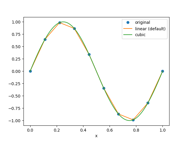
Interpolation methods
We use scipy.interpolate.interp1d() for 1-dimensional interpolation andscipy.interpolate.interpn() for multi-dimensional interpolation.
The interpolation method can be specified by the optional method argument.
- In [16]: da = xr.DataArray(np.sin(np.linspace(0, 2 * np.pi, 10)), dims='x',
- ....: coords={'x': np.linspace(0, 1, 10)})
- ....:
- In [17]: da.plot.line('o', label='original')
- Out[17]: [<matplotlib.lines.Line2D at 0x7f3425653710>]
- In [18]: da.interp(x=np.linspace(0, 1, 100)).plot.line(label='linear (default)')
- Out[18]: [<matplotlib.lines.Line2D at 0x7f34257677b8>]
- In [19]: da.interp(x=np.linspace(0, 1, 100), method='cubic').plot.line(label='cubic')
- Out[19]: [<matplotlib.lines.Line2D at 0x7f3425653470>]
- In [20]: plt.legend()
- Out[20]: <matplotlib.legend.Legend at 0x7f3424676c18>
 Additional keyword arguments can be passed to scipy’s functions.
- # fill 0 for the outside of the original coordinates.
- In [21]: da.interp(x=np.linspace(-0.5, 1.5, 10), kwargs={'fill_value': 0.0})
- Out[21]:
- <xarray.DataArray (x: 10)>
- array([ 0. , 0. , 0. , 0.813798, 0.604023, -0.604023,
- -0.813798, 0. , 0. , 0. ])
- Coordinates:
- * x (x) float64 -0.5 -0.2778 -0.05556 0.1667 ... 0.8333 1.056 1.278 1.5
- # extrapolation
- In [22]: da.interp(x=np.linspace(-0.5, 1.5, 10), kwargs={'fill_value': 'extrapolate'})
- Out[22]:
- <xarray.DataArray (x: 10)>
- array([-2.892544, -1.606969, -0.321394, 0.813798, 0.604023, -0.604023,
- -0.813798, 0.321394, 1.606969, 2.892544])
- Coordinates:
- * x (x) float64 -0.5 -0.2778 -0.05556 0.1667 ... 0.8333 1.056 1.278 1.5
Advanced Interpolation
interp() accepts DataArrayas similar to sel(), which enables us more advanced interpolation.Based on the dimension of the new coordinate passed to interp(), the dimension of the result are determined.
For example, if you want to interpolate a two dimensional array along a particular dimension, as illustrated below,you can pass two 1-dimensional DataArray s witha common dimension as new coordinate. For example:
- In [23]: da = xr.DataArray(np.sin(0.3 * np.arange(20).reshape(5, 4)),
- ....: [('x', np.arange(5)),
- ....: ('y', [0.1, 0.2, 0.3, 0.4])])
- ....:
- # advanced indexing
- In [24]: x = xr.DataArray([0, 2, 4], dims='z')
- In [25]: y = xr.DataArray([0.1, 0.2, 0.3], dims='z')
- In [26]: da.sel(x=x, y=y)
- Out[26]:
- <xarray.DataArray (z: 3)>
- array([ 0. , 0.42738 , -0.772764])
- Coordinates:
- x (z) int64 0 2 4
- y (z) float64 0.1 0.2 0.3
- Dimensions without coordinates: z
- # advanced interpolation
- In [27]: x = xr.DataArray([0.5, 1.5, 2.5], dims='z')
- In [28]: y = xr.DataArray([0.15, 0.25, 0.35], dims='z')
- In [29]: da.interp(x=x, y=y)
- Out[29]:
- <xarray.DataArray (z: 3)>
- array([ 0.556264, 0.634961, -0.466433])
- Coordinates:
- x (z) float64 0.5 1.5 2.5
- y (z) float64 0.15 0.25 0.35
- Dimensions without coordinates: z
where values on the original coordinates(x, y) = ((0.5, 0.15), (1.5, 0.25), (2.5, 0.35)) are obtained by the2-dimensional interpolation and mapped along a new dimension z.
If you want to add a coordinate to the new dimension z, you can supplyDataArray s with a coordinate,
- In [30]: x = xr.DataArray([0.5, 1.5, 2.5], dims='z', coords={'z': ['a', 'b','c']})
- In [31]: y = xr.DataArray([0.15, 0.25, 0.35], dims='z',
- ....: coords={'z': ['a', 'b','c']})
- ....:
- In [32]: da.interp(x=x, y=y)
- Out[32]:
- <xarray.DataArray (z: 3)>
- array([ 0.556264, 0.634961, -0.466433])
- Coordinates:
- x (z) float64 0.5 1.5 2.5
- y (z) float64 0.15 0.25 0.35
- * z (z) <U1 'a' 'b' 'c'
For the details of the advanced indexing,see more advanced indexing.
Interpolating arrays with NaN
Our interp() works with arrays with NaNthe same way thatscipy.interpolate.interp1d andscipy.interpolate.interpn do.linear and nearest methods return arrays including NaN,while other methods such as cubic or quadratic return all NaN arrays.
- In [33]: da = xr.DataArray([0, 2, np.nan, 3, 3.25], dims='x',
- ....: coords={'x': range(5)})
- ....:
- In [34]: da.interp(x=[0.5, 1.5, 2.5])
- Out[34]:
- <xarray.DataArray (x: 3)>
- array([ 1., nan, nan])
- Coordinates:
- * x (x) float64 0.5 1.5 2.5
- In [35]: da.interp(x=[0.5, 1.5, 2.5], method='cubic')
- Out[35]:
- <xarray.DataArray (x: 3)>
- array([nan, nan, nan])
- Coordinates:
- * x (x) float64 0.5 1.5 2.5
To avoid this, you can drop NaN by dropna(), andthen make the interpolation
- In [36]: dropped = da.dropna('x')
- In [37]: dropped
- Out[37]:
- <xarray.DataArray (x: 4)>
- array([0. , 2. , 3. , 3.25])
- Coordinates:
- * x (x) int64 0 1 3 4
- In [38]: dropped.interp(x=[0.5, 1.5, 2.5], method='cubic')
- Out[38]:
- <xarray.DataArray (x: 3)>
- array([1.190104, 2.507812, 2.929688])
- Coordinates:
- * x (x) float64 0.5 1.5 2.5
If NaNs are distributed randomly in your multidimensional array,dropping all the columns containing more than one NaNs bydropna() may lose a significant amount of information.In such a case, you can fill NaN by interpolate_na(),which is similar to pandas.Series.interpolate().
- In [39]: filled = da.interpolate_na(dim='x')
- In [40]: filled
- Out[40]:
- <xarray.DataArray (x: 5)>
- array([0. , 2. , 2.5 , 3. , 3.25])
- Coordinates:
- * x (x) int64 0 1 2 3 4
This fills NaN by interpolating along the specified dimension.After filling NaNs, you can interpolate:
- In [41]: filled.interp(x=[0.5, 1.5, 2.5], method='cubic')
- Out[41]:
- <xarray.DataArray (x: 3)>
- array([1.308594, 2.316406, 2.738281])
- Coordinates:
- * x (x) float64 0.5 1.5 2.5
For the details of interpolate_na(),see Missing values.
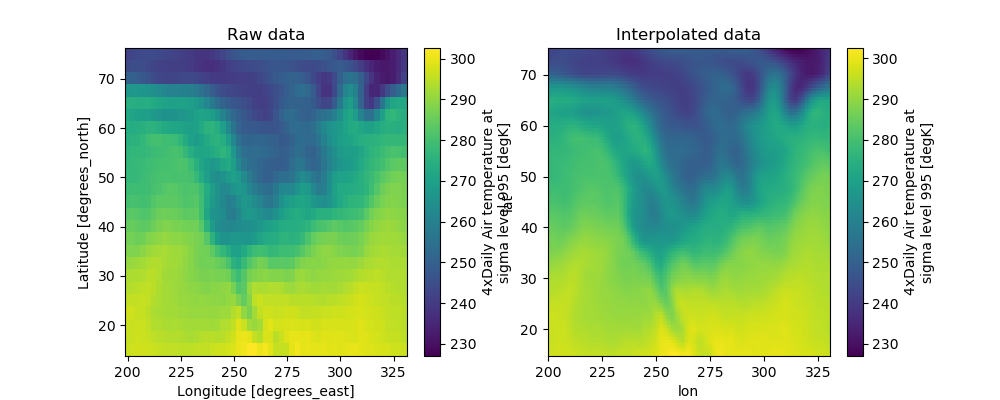
Example
Let’s see how interp() works on real data.
- # Raw data
- In [42]: ds = xr.tutorial.open_dataset('air_temperature').isel(time=0)
- In [43]: fig, axes = plt.subplots(ncols=2, figsize=(10, 4))
- In [44]: ds.air.plot(ax=axes[0])
- Out[44]: <matplotlib.collections.QuadMesh at 0x7f34255b9da0>
- In [45]: axes[0].set_title('Raw data')
- Out[45]: Text(0.5, 1.0, 'Raw data')
- # Interpolated data
- In [46]: new_lon = np.linspace(ds.lon[0], ds.lon[-1], ds.dims['lon'] * 4)
- In [47]: new_lat = np.linspace(ds.lat[0], ds.lat[-1], ds.dims['lat'] * 4)
- In [48]: dsi = ds.interp(lat=new_lat, lon=new_lon)
- In [49]: dsi.air.plot(ax=axes[1])
- Out[49]: <matplotlib.collections.QuadMesh at 0x7f3425426668>
- In [50]: axes[1].set_title('Interpolated data')
- Out[50]: Text(0.5, 1.0, 'Interpolated data')
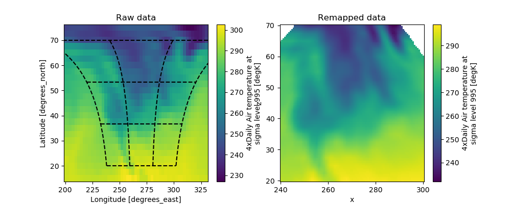
 Our advanced interpolation can be used to remap the data to the new coordinate.Consider the new coordinates x and z on the two dimensional plane.The remapping can be done as follows
- # new coordinate
- In [51]: x = np.linspace(240, 300, 100)
- In [52]: z = np.linspace(20, 70, 100)
- # relation between new and original coordinates
- In [53]: lat = xr.DataArray(z, dims=['z'], coords={'z': z})
- In [54]: lon = xr.DataArray((x[:, np.newaxis]-270)/np.cos(z*np.pi/180)+270,
- ....: dims=['x', 'z'], coords={'x': x, 'z': z})
- ....:
- In [55]: fig, axes = plt.subplots(ncols=2, figsize=(10, 4))
- In [56]: ds.air.plot(ax=axes[0])
- Out[56]: <matplotlib.collections.QuadMesh at 0x7f3424d20240>
- # draw the new coordinate on the original coordinates.
- In [57]: for idx in [0, 33, 66, 99]:
- ....: axes[0].plot(lon.isel(x=idx), lat, '--k')
- ....:
- In [58]: for idx in [0, 33, 66, 99]:
- ....: axes[0].plot(*xr.broadcast(lon.isel(z=idx), lat.isel(z=idx)), '--k')
- ....:
- In [59]: axes[0].set_title('Raw data')
- Out[59]: Text(0.5, 1.0, 'Raw data')
- In [60]: dsi = ds.interp(lon=lon, lat=lat)
- In [61]: dsi.air.plot(ax=axes[1])
- Out[61]: <matplotlib.collections.QuadMesh at 0x7f3424d46f60>
- In [62]: axes[1].set_title('Remapped data')
- Out[62]: Text(0.5, 1.0, 'Remapped data')