Parallel computing with Dask
xarray integrates with Dask to support parallelcomputations and streaming computation on datasets that don’t fit into memory.
Currently, Dask is an entirely optional feature for xarray. However, thebenefits of using Dask are sufficiently strong that Dask may become a requireddependency in a future version of xarray.
For a full example of how to use xarray’s Dask integration, read theblog post introducing xarray and Dask.
What is a Dask array?
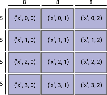 Dask divides arrays into many small pieces, called chunks, each of which ispresumed to be small enough to fit into memory.
Unlike NumPy, which has eager evaluation, operations on Dask arrays are lazy.Operations queue up a series of tasks mapped over blocks, and no computation isperformed until you actually ask values to be computed (e.g., to print resultsto your screen or write to disk). At that point, data is loaded into memoryand computation proceeds in a streaming fashion, block-by-block.
The actual computation is controlled by a multi-processing or thread pool,which allows Dask to take full advantage of multiple processors available onmost modern computers.
For more details on Dask, read its documentation.
Reading and writing data
The usual way to create a dataset filled with Dask arrays is to load thedata from a netCDF file or files. You can do this by supplying a chunksargument to open_dataset() or using theopen_mfdataset() function.
- In [1]: ds = xr.open_dataset('example-data.nc', chunks={'time': 10})
- In [2]: ds
- Out[2]:
- <xarray.Dataset>
- Dimensions: (latitude: 180, longitude: 360, time: 365)
- Coordinates:
- * time (time) datetime64[ns] 2015-01-01 2015-01-02 ... 2015-12-31
- * longitude (longitude) int64 0 1 2 3 4 5 6 ... 353 354 355 356 357 358 359
- * latitude (latitude) float64 89.5 88.5 87.5 86.5 ... -87.5 -88.5 -89.5
- Data variables:
- temperature (time, latitude, longitude) float64 dask.array<shape=(365, 180, 360), chunksize=(10, 180, 360)>
In this example latitude and longitude do not appear in the chunksdict, so only one chunk will be used along those dimensions. It is alsoentirely equivalent to opening a dataset using open_dataset and thenchunking the data using the chunk method, e.g.,xr.open_dataset('example-data.nc').chunk({'time': 10}).
To open multiple files simultaneously, use open_mfdataset():
- xr.open_mfdataset('my/files/*.nc')
This function will automatically concatenate and merge dataset into one inthe simple cases that it understands (see auto_combine()for the full disclaimer). By default, open_mfdataset will chunk eachnetCDF file into a single Dask array; again, supply the chunks argument tocontrol the size of the resulting Dask arrays. In more complex cases, you canopen each file individually using open_dataset and merge the result, asdescribed in Combining data.
You’ll notice that printing a dataset still shows a preview of array values,even if they are actually Dask arrays. We can do this quickly with Dask becausewe only need to compute the first few values (typically from the first block).To reveal the true nature of an array, print a DataArray:
- In [3]: ds.temperature
- Out[3]:
- <xarray.DataArray 'temperature' (time: 365, latitude: 180, longitude: 360)>
- dask.array<shape=(365, 180, 360), dtype=float64, chunksize=(10, 180, 360)>
- Coordinates:
- * time (time) datetime64[ns] 2015-01-01 2015-01-02 ... 2015-12-31
- * longitude (longitude) int64 0 1 2 3 4 5 6 7 ... 353 354 355 356 357 358 359
- * latitude (latitude) float64 89.5 88.5 87.5 86.5 ... -87.5 -88.5 -89.5
Once you’ve manipulated a Dask array, you can still write a dataset too big tofit into memory back to disk by using to_netcdf() in theusual way.
- In [4]: ds.to_netcdf('manipulated-example-data.nc')
By setting the compute argument to False, to_netcdf()will return a Dask delayed object that can be computed later.
- In [5]: from dask.diagnostics import ProgressBar
- # or distributed.progress when using the distributed scheduler
- In [6]: delayed_obj = ds.to_netcdf('manipulated-example-data.nc', compute=False)
- In [7]: with ProgressBar():
- ...: results = delayed_obj.compute()
- ...:
- [ ] | 0% Completed | 0.0s
- [## ] | 5% Completed | 0.2s
- [################### ] | 48% Completed | 0.3s
- [################################### ] | 88% Completed | 0.4s
- [####################################### ] | 98% Completed | 1.3s
- [########################################] | 100% Completed | 1.4s
Note
When using Dask’s distributed scheduler to write NETCDF4 files,it may be necessary to set the environment variable HDF5_USE_FILE_LOCKING=FALSE_to avoid competing locks within the HDF5 SWMR file locking scheme. Note thatwriting netCDF files with Dask’s distributed scheduler is only supported forthe _netcdf4 backend.
A dataset can also be converted to a Dask DataFrame using to_dask_dataframe().
- In [8]: df = ds.to_dask_dataframe()
- In [9]: df
- Out[9]:
- Dask DataFrame Structure:
- latitude longitude time temperature
- npartitions=44
- 0 float64 int64 datetime64[ns] float64
- 525600 ... ... ... ...
- ... ... ... ... ...
- 22600800 ... ... ... ...
- 23651999 ... ... ... ...
- Dask Name: concat-indexed, 1481 tasks
Dask DataFrames do not support multi-indexes so the coordinate variables from the dataset are included as columns in the Dask DataFrame.
Using Dask with xarray
Nearly all existing xarray methods (including those for indexing, computation,concatenating and grouped operations) have been extended to work automaticallywith Dask arrays. When you load data as a Dask array in an xarray datastructure, almost all xarray operations will keep it as a Dask array; when thisis not possible, they will raise an exception rather than unexpectedly loadingdata into memory. Converting a Dask array into memory generally requires anexplicit conversion step. One notable exception is indexing operations: toenable label based indexing, xarray will automatically load coordinate labelsinto memory.
The easiest way to convert an xarray data structure from lazy Dask arrays intoeager, in-memory NumPy arrays is to use the load() method:
- In [10]: ds.load()
- Out[10]:
- <xarray.Dataset>
- Dimensions: (latitude: 180, longitude: 360, time: 365)
- Coordinates:
- * time (time) datetime64[ns] 2015-01-01 2015-01-02 ... 2015-12-31
- * longitude (longitude) int64 0 1 2 3 4 5 6 ... 353 354 355 356 357 358 359
- * latitude (latitude) float64 89.5 88.5 87.5 86.5 ... -87.5 -88.5 -89.5
- Data variables:
- temperature (time, latitude, longitude) float64 0.4691 -0.2829 ... 0.005886
You can also access values, which will always be aNumPy array:
- In [11]: ds.temperature.values
- Out[11]:
- array([[[ 4.691e-01, -2.829e-01, ..., -5.577e-01, 3.814e-01],
- [ 1.337e+00, -1.531e+00, ..., 8.726e-01, -1.538e+00],
- ...
- # truncated for brevity
Explicit conversion by wrapping a DataArray with np.asarray also works:
- In [12]: np.asarray(ds.temperature)
- Out[12]:
- array([[[ 4.691e-01, -2.829e-01, ..., -5.577e-01, 3.814e-01],
- [ 1.337e+00, -1.531e+00, ..., 8.726e-01, -1.538e+00],
- ...
Alternatively you can load the data into memory but keep the arrays asDask arrays using the persist() method:
- In [13]: ds = ds.persist()
This is particularly useful when using a distributed cluster because the datawill be loaded into distributed memory across your machines and be much fasterto use than reading repeatedly from disk. Warning that on a single machinethis operation will try to load all of your data into memory. You should makesure that your dataset is not larger than available memory.
For performance you may wish to consider chunk sizes. The correct choice ofchunk size depends both on your data and on the operations you want to perform.With xarray, both converting data to a Dask arrays and converting the chunksizes of Dask arrays is done with the chunk() method:
- In [14]: rechunked = ds.chunk({'latitude': 100, 'longitude': 100})
You can view the size of existing chunks on an array by viewing thechunks attribute:
- In [15]: rechunked.chunks
- Out[15]: Frozen(SortedKeysDict({'time': (10, 10, 10, 10, 10, 10, 10, 10, 10, 10, 10, 10, 10, 10, 10, 10, 10, 10, 10, 10, 10, 10, 10, 10, 10, 10, 10, 10, 10, 10, 10, 10, 10, 10, 10, 10, 5), 'latitude': (100, 80), 'longitude': (100, 100, 100, 60)}))
If there are not consistent chunksizes between all the arrays in a datasetalong a particular dimension, an exception is raised when you try to access.chunks.
Note
In the future, we would like to enable automatic alignment of Daskchunksizes (but not the other way around). We might also require that allarrays in a dataset share the same chunking alignment. Neither of theseare currently done.
NumPy ufuncs like np.sin currently only work on eagerly evaluated arrays(this will change with the next major NumPy release). We have providedreplacements that also work on all xarray objects, including those that storelazy Dask arrays, in the xarray.ufuncs module:
- In [16]: import xarray.ufuncs as xu
- In [17]: xu.sin(rechunked)
- Out[17]:
- <xarray.Dataset>
- Dimensions: (latitude: 180, longitude: 360, time: 365)
- Coordinates:
- * time (time) datetime64[ns] 2015-01-01 2015-01-02 ... 2015-12-31
- * longitude (longitude) int64 0 1 2 3 4 5 6 ... 353 354 355 356 357 358 359
- * latitude (latitude) float64 89.5 88.5 87.5 86.5 ... -87.5 -88.5 -89.5
- Data variables:
- temperature (time, latitude, longitude) float64 dask.array<shape=(365, 180, 360), chunksize=(10, 100, 100)>
To access Dask arrays directly, use the newDataArray.data attribute. This attribute exposesarray data either as a Dask array or as a NumPy array, depending on whether it has beenloaded into Dask or not:
- In [18]: ds.temperature.data
- Out[18]: dask.array<xarray-temperature, shape=(365, 180, 360), dtype=float64, chunksize=(10, 180, 360)>
Note
In the future, we may extend .data to support other “computable” arraybackends beyond Dask and NumPy (e.g., to support sparse arrays).
Automatic parallelization
Almost all of xarray’s built-in operations work on Dask arrays. If you want touse a function that isn’t wrapped by xarray, one option is to extract Daskarrays from xarray objects (.data) and use Dask directly.
Another option is to use xarray’s apply_ufunc(), which canautomate embarrassingly parallel “map” type operationswhere a function written for processing NumPy arrays should be repeatedlyapplied to xarray objects containing Dask arrays. It works similarly todask.array.map_blocks() and dask.array.atop(), but withoutrequiring an intermediate layer of abstraction.
For the best performance when using Dask’s multi-threaded scheduler, wrap afunction that already releases the global interpreter lock, which fortunatelyalready includes most NumPy and Scipy functions. Here we show an exampleusing NumPy operations and a fast function frombottleneck, whichwe use to calculate Spearman’s rank-correlation coefficient:
- import numpy as np
- import xarray as xr
- import bottleneck
- def covariance_gufunc(x, y):
- return ((x - x.mean(axis=-1, keepdims=True))
- * (y - y.mean(axis=-1, keepdims=True))).mean(axis=-1)
- def pearson_correlation_gufunc(x, y):
- return covariance_gufunc(x, y) / (x.std(axis=-1) * y.std(axis=-1))
- def spearman_correlation_gufunc(x, y):
- x_ranks = bottleneck.rankdata(x, axis=-1)
- y_ranks = bottleneck.rankdata(y, axis=-1)
- return pearson_correlation_gufunc(x_ranks, y_ranks)
- def spearman_correlation(x, y, dim):
- return xr.apply_ufunc(
- spearman_correlation_gufunc, x, y,
- input_core_dims=[[dim], [dim]],
- dask='parallelized',
- output_dtypes=[float])
The only aspect of this example that is different from standard usage ofapply_ufunc() is that we needed to supply the output_dtypes arguments.(Read up on Wrapping custom computation for an explanation of the“core dimensions” listed in input_core_dims.)
Our new spearman_correlation() function achieves near linear speedupwhen run on large arrays across the four cores on my laptop. It would alsowork as a streaming operation, when run on arrays loaded from disk:
- In [19]: rs = np.random.RandomState(0)
- In [20]: array1 = xr.DataArray(rs.randn(1000, 100000), dims=['place', 'time']) # 800MB
- In [21]: array2 = array1 + 0.5 * rs.randn(1000, 100000)
- # using one core, on NumPy arrays
- In [22]: %time _ = spearman_correlation(array1, array2, 'time')
- CPU times: user 21.6 s, sys: 2.84 s, total: 24.5 s
- Wall time: 24.9 s
- In [23]: chunked1 = array1.chunk({'place': 10})
- In [24]: chunked2 = array2.chunk({'place': 10})
- # using all my laptop's cores, with Dask
- In [25]: r = spearman_correlation(chunked1, chunked2, 'time').compute()
- In [26]: %time _ = r.compute()
- CPU times: user 30.9 s, sys: 1.74 s, total: 32.6 s
- Wall time: 4.59 s
One limitation of apply_ufunc() is that it cannot be applied to arrays withmultiple chunks along a core dimension:
- In [27]: spearman_correlation(chunked1, chunked2, 'place')
- ValueError: dimension 'place' on 0th function argument to apply_ufunc with
- dask='parallelized' consists of multiple chunks, but is also a core
- dimension. To fix, rechunk into a single Dask array chunk along this
- dimension, i.e., ``.rechunk({'place': -1})``, but beware that this may
- significantly increase memory usage.
This reflects the nature of core dimensions, in contrast to broadcast (non-core)dimensions that allow operations to be split into arbitrary chunks forapplication.
Tip
For the majority of NumPy functions that are already wrapped by Dask, it’susually a better idea to use the pre-existing dask.array function, byusing either a pre-existing xarray methods orapply_ufunc() with dask='allowed'. Dask can oftenhave a more efficient implementation that makes use of the specializedstructure of a problem, unlike the generic speedups offered bydask='parallelized'.
Chunking and performance
The chunks parameter has critical performance implications when using Daskarrays. If your chunks are too small, queueing up operations will be extremelyslow, because Dask will translate each operation into a huge number ofoperations mapped across chunks. Computation on Dask arrays with small chunkscan also be slow, because each operation on a chunk has some fixed overhead fromthe Python interpreter and the Dask task executor.
Conversely, if your chunks are too big, some of your computation may be wasted,because Dask only computes results one chunk at a time.
A good rule of thumb is to create arrays with a minimum chunksize of at leastone million elements (e.g., a 1000x1000 matrix). With large arrays (10+ GB), thecost of queueing up Dask operations can be noticeable, and you may need evenlarger chunksizes.
Optimization Tips
With analysis pipelines involving both spatial subsetting and temporal resampling, Dask performance can become very slow in certain cases. Here are some optimization tips we have found through experience:
Do your spatial and temporal indexing (e.g.
.sel()or.isel()) early in the pipeline, especially before callingresample()orgroupby(). Grouping and resampling triggers some computation on all the blocks, which in theory should commute with indexing, but this optimization hasn’t been implemented in Dask yet. (See Dask issue #746).Save intermediate results to disk as a netCDF files (using
to_netcdf()) and then load them again withopen_dataset()for further computations. For example, if subtracting temporal mean from a dataset, save the temporal mean to disk before subtracting. Again, in theory, Dask should be able to do the computation in a streaming fashion, but in practice this is a fail case for the Dask scheduler, because it tries to keep every chunk of an array that it computes in memory. (See Dask issue #874)Specify smaller chunks across space when using
open_mfdataset()(e.g.,chunks={'latitude': 10, 'longitude': 10}). This makes spatial subsetting easier, because there’s no risk you will load chunks of data referring to different chunks (probably not necessary if you follow suggestion 1).