
1.3.2.2 基础简化
1.3.2.2.1 计算求和
In [79]:
x = np.array([1, 2, 3, 4])np.sum(x)
Out[79]:
10
In [80]:
x.sum()
Out[80]:
10
行求和和列求和:

In [81]:
x = np.array([[1, 1], [2, 2]])x
Out[81]:
array([[1, 1],[2, 2]])
In [83]:
x.sum(axis=0) # 列 (第一纬度)
Out[83]:
array([3, 3])
In [84]:
x[:, 0].sum(), x[:, 1].sum()
Out[84]:
(3, 3)
In [85]:
x.sum(axis=1) # 行 (第二纬度)
Out[85]:
array([2, 4])
In [86]:
x[0, :].sum(), x[1, :].sum()
Out[86]:
(2, 4)
相同的思路在高维:
In [87]:
x = np.random.rand(2, 2, 2)x.sum(axis=2)[0, 1]
Out[87]:
1.2671177193964822
In [88]:
x[0, 1, :].sum()
Out[88]:
1.2671177193964822
1.3.2.2.2 其他简化
- 以相同方式运作(也可以使用
axis=)
极值
In [89]:
x = np.array([1, 3, 2])x.min()
Out[89]:
1
In [90]:
x.max()
Out[90]:
3
In [91]:
x.argmin() # 最小值的索引
Out[91]:
0
In [92]:
x.argmax() # 最大值的索引
Out[92]:
1
逻辑运算:
In [93]:
np.all([True, True, False])
Out[93]:
False
In [94]:
np.any([True, True, False])
Out[94]:
True
注:可以被应用数组对比:
In [95]:
a = np.zeros((100, 100))np.any(a != 0)
Out[95]:
False
In [96]:
np.all(a == a)
Out[96]:
True
In [97]:
a = np.array([1, 2, 3, 2])b = np.array([2, 2, 3, 2])c = np.array([6, 4, 4, 5])((a <= b) & (b <= c)).all()
Out[97]:
True
统计:
In [98]:
x = np.array([1, 2, 3, 1])y = np.array([[1, 2, 3], [5, 6, 1]])x.mean()
Out[98]:
1.75
In [99]:
np.median(x)
Out[99]:
1.5
In [100]:
np.median(y, axis=-1) # 最后的坐标轴
Out[100]:
array([ 2., 5.])
In [101]:
x.std() # 全体总体的标准差。
Out[101]:
0.82915619758884995
… 以及其他更多(随着你成长最好学习一下)。
练习:简化
- 假定有
sum,你会期望看到哪些其他的函数? sum和cumsum有什么区别?
实例: 数据统计
populations.txt中的数据描述了过去20年加拿大北部野兔和猞猁的数量(以及胡萝卜)。
你可以在编辑器或在IPython看一下数据(shell或者notebook都可以):
In [104]:
cat data/populations.txt
# year hare lynx carrot1900 30e3 4e3 483001901 47.2e3 6.1e3 482001902 70.2e3 9.8e3 415001903 77.4e3 35.2e3 382001904 36.3e3 59.4e3 406001905 20.6e3 41.7e3 398001906 18.1e3 19e3 386001907 21.4e3 13e3 423001908 22e3 8.3e3 445001909 25.4e3 9.1e3 421001910 27.1e3 7.4e3 460001911 40.3e3 8e3 468001912 57e3 12.3e3 438001913 76.6e3 19.5e3 409001914 52.3e3 45.7e3 394001915 19.5e3 51.1e3 390001916 11.2e3 29.7e3 367001917 7.6e3 15.8e3 418001918 14.6e3 9.7e3 433001919 16.2e3 10.1e3 413001920 24.7e3 8.6e3 47300
首先,将数据加载到Numpy数组:
In [107]:
data = np.loadtxt('data/populations.txt')year, hares, lynxes, carrots = data.T # 技巧: 将列分配给变量
接下来作图:
In [108]:
from matplotlib import pyplot as pltplt.axes([0.2, 0.1, 0.5, 0.8])plt.plot(year, hares, year, lynxes, year, carrots)plt.legend(('Hare', 'Lynx', 'Carrot'), loc=(1.05, 0.5))
Out[108]:
<matplotlib.legend.Legend at 0x1070407d0>
随时间变化的人口平均数:
In [109]:
populations = data[:, 1:]populations.mean(axis=0)
Out[109]:
array([ 34080.95238095, 20166.66666667, 42400\. ])
样本的标准差:
In [110]:
populations.std(axis=0)
Out[110]:
array([ 20897.90645809, 16254.59153691, 3322.50622558])
每一年哪个物种有最高的人口?:
In [111]:
np.argmax(populations, axis=1)
Out[111]:
array([2, 2, 0, 0, 1, 1, 2, 2, 2, 2, 2, 2, 0, 0, 0, 1, 2, 2, 2, 2, 2])
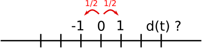
实例:随机游走算法扩散
让我们考虑一下简单的1维随机游走过程:在每个时间点,行走者以相等的可能性跳到左边或右边。我们感兴趣的是找到随机游走者在 t 次左跳或右跳后距离原点的典型距离?我们将模拟许多”行走者“来找到这个规律,并且我们将采用数组计算技巧来计算:我们将创建一个2D数组记录事实,一个方向是经历(每个行走者有一个经历),一个纬度是时间:
In [113]:
n_stories = 1000 # 行走者的数t_max = 200 # 我们跟踪行走者的时间
我们随机选择步长1或-1去行走:
In [115]:
t = np.arange(t_max)steps = 2 * np.random.random_integers(0, 1, (n_stories, t_max)) - 1np.unique(steps) # 验证: 所有步长是1或-1
Out[115]:
array([-1, 1])
我们通过汇总随着时间的步骤来构建游走
In [116]:
positions = np.cumsum(steps, axis=1) # axis = 1: 纬度是时间sq_distance = positions**2
获得经历轴的平均数:
In [117]:
mean_sq_distance = np.mean(sq_distance, axis=0)
画出结果:
In [126]:
plt.figure(figsize=(4, 3))plt.plot(t, np.sqrt(mean_sq_distance), 'g.', t, np.sqrt(t), 'y-')plt.xlabel(r"$t$")plt.ylabel(r"$\sqrt{\langle (\delta x)^2 \rangle}$")
Out[126]:
<matplotlib.text.Text at 0x10b529450>
我们找到了物理学上一个著名的结果:均方差记录是时间的平方根!


